Education pays off (for the state too): net fiscal contributions by educational attainment in Spain

Introduction
When people argue about the fiscal sustainability of the welfare state, they are (often implicitly) arguing about a simple accounting identity: some individuals receive more from the state than they pay in, and others pay more than they receive. The key questions are how large those gaps are, when they occur over the life cycle, and how they differ across groups. These underpin debates about the returns to public investment in education, the sustainability of pension systems, and — perhaps more controversially — the fiscal impact of immigration from countries with different educational profiles.
This post constructs net fiscal contribution (NFC) profiles by educational attainment for Spain, following the National Transfer Accounts (NTA) methodology.
Methodology overview
The NTA framework provides a standardised approach for measuring economic flows across generations. The core idea is simple: at each age, individuals receive certain benefits from the state (transfer inflows) and contribute to the state through taxes (transfer outflows). The difference between these (the net fiscal contribution) tells us whether a given age group is a net contributor or net recipient.
$$ \text{NFC}(a,e) = \text{Outflows}(a,e) - \text{Inflows}(a,e) $$
where $a$ denotes age and $e$ denotes educational attainment. A positive NFC means the individual contributes more than they receive, whereas a negative NFC means they are a net recipient.
Data
The analysis draws on the following datasets:
ES-SILC (ECV): The microdata for the 2024 wave of Spain's Survey of Living Conditions (i.e., the Spanish EU-SILC), which provides individual-level data on earnings, benefits and socio-demographic characteristics.
Eurostat national accounts: Macro control totals for rescaling survey-based estimates to match official statistics:
nama_10_gdp: GDP components including household final consumption expenditure and government consumptiongov_10a_main: Government sector accountsgov_10a_exp: Government expenditure by function
Eurostat education finance data: Public expenditure per student by education level (
educ_uoe_fine09)DG TAXUD data on aggregate tax revenues
European NTA consumption profiles: Pre-computed age profiles of public and private consumption by category for Spain
Educational attainment is coded using the ISCED 2011 classification. The table below shows the mapping from ISCED levels to the categories used in the analysis.
| ISCED level | Description | Category |
|---|---|---|
| 0 | Early childhood education | Pre-primary |
| 1 | Primary education | Primary |
| 2 | Lower secondary education | Lower secondary |
| 3–4 | Upper secondary and post-secondary non-tertiary | Upper secondary |
| 5–8 | Tertiary education | Tertiary |
For the final results, I aggregate to three broad categories to ensure adequate cell sizes at each age: Primary or less (ISCED 0–1), Secondary (ISCED 2–4), and Tertiary (ISCED 5–8).
Transfer inflows
Transfer inflows consist of two main components: cash benefits received from the government and public consumption (the value of in-kind public services consumed).
Cash benefits
Cash benefits are measured from household survey microdata both at the individual level (for personal benefits) and at the household level (for household-level transfers). Individual-level benefits include unemployment benefits, old-age pensions, survivor benefits, sickness benefits, disability benefits, and education-related benefits. Household-level benefits (which include housing allowances, family/child allowances, and social exclusion benefits) are divided equally among household members.
I aggregate all cash benefits to the individual level and then rescale to match the national accounts macro control for social benefits other than social transfers in-kind paid by the general government (D62 from gov_10a_main):
$$ B_i^{\text{scaled}} = B_i^{\text{survey}} \times \frac{\text{D62}}{\sum_i B_i^{\text{survey}} \times w_i} $$
where $w_i$ are the survey weights.
Public consumption
Public consumption represents the value of government-provided services consumed by individuals. I decompose this into two components: public education ($G^E$) and other public consumption ($G^O$, which includes healthcare and general government services).
Other public consumption (healthcare and general services)
For healthcare and other government services, consumption is allocated using pre-computed age profiles for Spain from the European NTA. These profiles capture the well-documented pattern of healthcare consumption rising sharply with age.
Other public consumption is not differentiated by education — the assumption is that individuals of the same age consume similar amounts of healthcare and other public services regardless of their educational attainment.1
The profiles are rescaled so that the population-weighted total matches the macro control for non-education government consumption:
$$ G^O_{\text{macro}} = \text{P3\_S13} - \text{GF09} $$
where P3_S13 is total government consumption from the national accounts and GF09 is final government consumption expenditure on education from COFOG.
Public education consumption
Education consumption requires different treatment because it varies systematically with educational attainment: a university graduate received substantially more public investment during their schooling years than someone who left after compulsory education.
The allocation procedure rests on two building blocks:
- Enrolment data: I gather data on per-student costs by education level (
educ_uoe_fine09). Since the latest available data is for 2022, I adjust it to 2023 prices using the government consumption deflator. - Macro control: Final government consumption expenditure on education from COFOG (GF09 in
gov_10a_exp), which the individual-level allocations must sum to.
For each individual in the survey, I assign education consumption as follows. For individuals currently enrolled in education, I assign consumption based on their enrolment level and the corresponding per-student cost. For children under 16, I impute current enrollment based on age (see table below). Individuals not currently enrolled receive zero education consumption.
| Age | Imputed enrollment |
|---|---|
| 0-2 | Not enrolled |
| 3-5 | Pre-primary |
| 6-11 | Primary |
| 12-15 | Lower secondary |
Finally, I rescale all values proportionally so that the population-weighted total matches the COFOG macro control.
Transfer outflows
Transfer outflows consist of taxes paid. Following the NTA methodology, I decompose total taxes into three components: taxes on labour income, taxes on capital income, and taxes on consumption.
Two features of the Spanish tax system require careful treatment when constructing education-specific income tax profiles. First, Spain has a progressive tax system: higher earners face higher marginal rates and pay a larger share of their income in taxes. The standard NTA approach takes gross income from surveys and rescales uniformly to match macro tax aggregates, implicitly assuming a flat tax rate across the income distribution. Since educational attainment is strongly correlated with earnings, ignoring progressivity would compress differences across education groups — understating the tax burden of higher-educated individuals and overstating that of lower-educated individuals.
Second, most cash transfers in Spain are subject to personal income tax. Recall that transfer inflows are measured as gross government expenditure (i.e., the full amount the state disburses). But recipients do not keep all of this: pensions, unemployment benefits, and most other social transfers enter the tax base and are taxed according to the standard rate schedule. These taxes paid on benefits must appear somewhere in transfer outflows. Indeed, the DG TAXUD classification allocates taxes on pensions and social transfers to "taxes on non-employed labour income", a subcategory of labour taxes. A methodology that only considers taxes on earnings would miss this component, understating the tax contributions of groups that receive substantial taxable transfers (particularly retirees).
To address both issues, I exploit the fact that the ES-SILC reports both gross and net income variables. The difference between gross and net income captures the actual tax incidence as reported in the survey, which already incorporates the progressive rate structure and taxes paid on benefits:
$$ T_i^{\text{survey}} = Y_i^{\text{gross}} - Y_i^{\text{net}} $$
This survey-based tax amount is then rescaled to match macro controls:
$$ T_i^{\text{scaled}} = T_i^{\text{survey}} \times \frac{T_{\text{agg}}}{\sum_i T_i^{\text{survey}} \times w_i} $$
This approach preserves the shape of the tax profile (reflecting both progressivity and the taxation of transfers) while ensuring consistency with national accounts.
Labour income taxes
Gross labour income in the survey comprises gross cash earnings from employment, non-cash employee income (including company car) and employer social security contributions. Gross benefit income includes unemployment benefits, old-age pensions, survivor benefits, sickness and disability benefits, and education-related allowances. Self-employment income is treated separately.
Net income is constructed analogously from the corresponding net variables. The implied tax on each component is the difference between gross and net totals:
$$ T^L_i = Y^{L,\text{gross}}_i - Y^{L,\text{net}}_i \quad ; \quad T^{SE}_i = Y^{SE,\text{gross}}_i - Y^{SE,\text{net}}_i \quad ; \quad T^B_i = B^{\text{gross}}_i - B^{\text{net}}_i $$
Each component is rescaled to its corresponding DG TAXUD macro control: employment taxes to taxes on income form employment, benefit taxes to taxes paid by the non-employed (which captures taxes on pensions and social transfers), and self-employment taxes to taxes on income of self-employed.
Capital income taxes
Capital income is measured at the household level and includes interest, dividends, profit from capital investments, and rental income. I compute implied capital taxes as the difference between gross and net capital income at the household level and allocate this to the household head. The profile is rescaled to the DG TAXUD aggregate for capital taxes on household and corporate income, excluding the self-employment component (which is treated as labour above).
Consumption taxes
Consumption taxes present a different challenge. The standard NTA approach allocates consumption taxes based on age-specific consumption profiles without further disaggregation, but total consumption varies systematically with income — and hence with educational attainment.
I start from pre-computed age profiles of private consumption for Spain from the European NTA. These profiles are uniform across education groups, so I adjust them to reflect income-related differences in consumption. I compute mean disposable income by age-education cell and define an adjustment factor:
$$\alpha(a,e) = \left(\frac{\bar{Y}(a,e)}{\bar{Y}}\right)^{\gamma}$$
where $\gamma < 1$ captures the concavity of the consumption-income relationship. I set $\gamma = 0.6$, which implies that a doubling of income increases consumption by approximately 50% — consistent with empirical estimates of the income elasticity of consumption.2 The base consumption profile is multiplied by this adjustment factor to generate education-specific profiles, which are then rescaled so that the population-weighted total matches the national accounts aggregate for household consumption. Consumption taxes are allocated in proportion to consumption, with the aggregate matching DG TAXUD data on consumption tax revenue.
Combining inflows and outflows
For each individual, I compute the net fiscal contribution as:
$$ \text{NFC}_i = T^L_i + T^K_i + T^C_i - B_i - G_i $$
I then compute weighted means by age and education level to construct the final profiles, which are smoothed using a local polynomial regression (LOESS).
Handling empty cells at young ages
A methodological challenge arises when constructing profiles by educational attainment: at young ages, cells for higher attainment levels are not defined. Educational attainment is a stock variable observed at the time of the survey, whereas fiscal flows occur throughout the life cycle. For a child currently in school, we observe their eventual educational attainment in the cross-section, but their current fiscal profile is largely independent of that future attainment. For visualization purposes, I compute population-weighted per capita values by age, pooling across education categories, and apply this uniform value to all education groups at ages where education-specific estimation is not conceptually feasible. As a result, the final profiles diverge only at ages where economic behaviour genuinely differs by attainment — typically from the late teens onwards. This ensures that the childhood portions of the profiles are identical across education groups.
Results
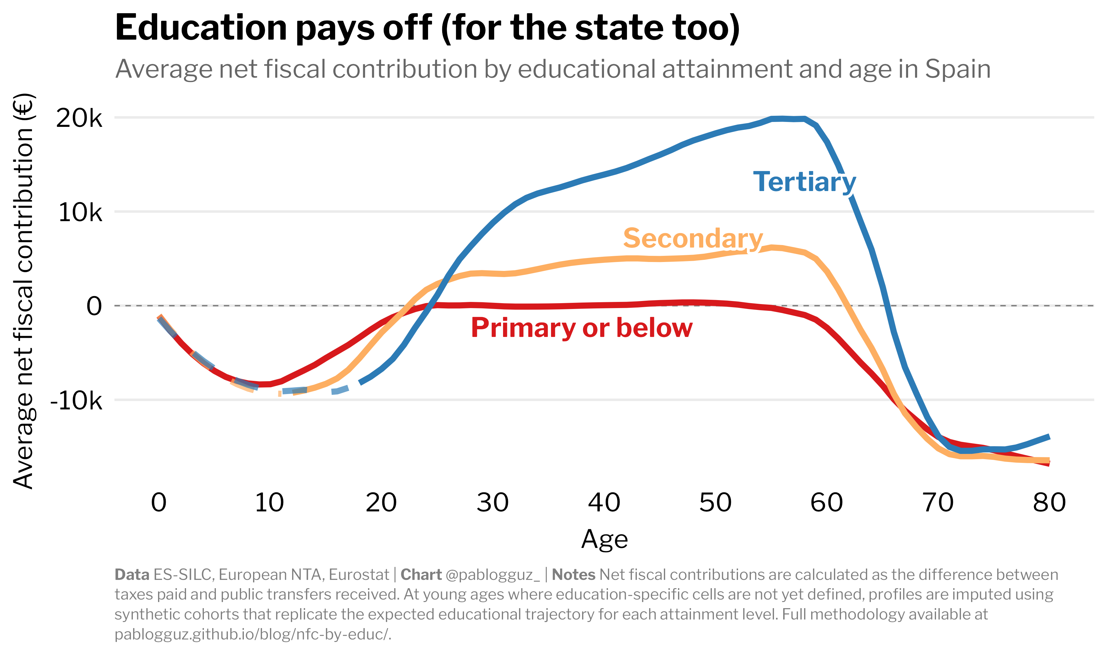
These profiles highlight that the fiscal position of an individual is shaped by two interacting margins: (i) where they sit in the life cycle, and (ii) the earning capacity associated with their skills and education. The life-cycle pattern is common across groups (net receipts in childhood, net payments during working ages, and net receipts in retirement) but the height and width of the contribution window differ sharply by educational attainment.
Tertiary-educated graduates are net fiscal contributors from their late 20s until their mid-60s, with average contributions around €13,000 per year during prime working ages (25-54). After retirement, they become net recipients, but their implied synthetic lifetime contributions remain positive. Those with secondary education are also net fiscal contributors during their working lives, but with more modest average contributions during prime working ages (of the order of one-third of the average for tertiary-educated individuals). However, their synthetic lifetime fiscal contribution turns negative once we account for receipts during childhood and retirement.
Those with only primary education or below are roughly neutral for most of their working lives: even during prime working ages, their average net fiscal contribution is close to zero. As a result, their synthetic lifetime fiscal contribution is substantially negative.
An important part of these gaps stems from differences in labour market attachment. In the survey, prime working-age individuals with less than secondary education have an employment rate of around 55%, compared to over 85% for those with tertiary education. Interestingly, the employment rate of individuals with tertiary education aged 60-64 is above the prime working-age employment rate of those with only primary education.
Caveats
This exercise constructs period (cross-sectional) NFC profiles by age and educational attainment. It does not follow the same people over time, and it does not observe the full fiscal life cycle of any cohort. Instead, it combines a snapshot of age-specific flows observed (or imputed) in one year. That is standard in the NTA tradition, but it comes with important limitations.
Age profiles are “period” profiles, not cohort histories. At a given age, the tertiary-educated individuals observed in the 2024 survey are not the same people as the tertiary-educated individuals observed at age 60. Cohorts differ in lifetime earnings paths, labour-market attachment, and institutional exposure. As a result, these profiles should be read as: “How much do 40-year-olds with tertiary education contribute/receive under today’s institutions and macro aggregates?”, but not as “What will today’s 40-year-olds experience when they are 60?”. In other words, any implied lifetime contribution computed by integrating these cross-sectional profiles is a synthetic construct that reflects the current fiscal architecture rather than a prediction of future net contributions.
Educational attainment is not exogenous. Differences in NFC across education groups should not be interpreted causally as the fiscal return to education but simply as an accounting decomposition.
In sum, the results are best interpreted as a consistent, macro-anchored snapshot of who pays and who receives today, by age and education, under current institutions. They are informative for understanding the structure of fiscal redistribution, but they are not a cohort forecast and should not be read as a causal estimate of the fiscal payoff to schooling.
This is a strong assumption. Whereas one should be less worried about collective consumption (e.g. street lighting), healthcare consumption likely varies with socio-economic status. However, it can go either way as two forces pull in opposite directions: on the one hand, lower-educated individuals tend to have worse health outcomes and thus may have more need and often more acute/inpatient use; on the other hand, higher-educated individuals may use more preventive and specialist/outpatient care conditional on need. For the purpose of this exercise I abstract from this heterogeneity, but it is a limitation to keep in mind.