No country for young men: age-earnings profiles by birth cohort and sex in Spain

2025-10-09

8 minute read

Introduction#

Spain's younger generations are not enjoying higher wages than their parents did at the same age. In fact, each successive male cohort since the 1960s appears to do progressively worse: men born in the 1990s, now in their mid-30s, earn about 9% less in real terms than men born in the 1970s at comparable ages.

Women's wage trajectories tell a different story: recent cohorts have achieved parity with earlier generations and appear on track to surpass them. While matching or slightly exceeding wage levels from decades ago is hardly cause for celebration, it stands in marked contrast to the persistent declines young men have experienced.

This post documents an attempt to construct age-earnings profiles by birth cohort in Spain. My approach accounts for methodological breaks in the underlying survey data and allows me to track different generations across their working lives.

Data#

The main analysis draws on the following datasets, all publicly available:

Structure of Earnings Survey: Estimates of average gross wages by age group and sex. My analysis includes the annual surveys from 2004-07 and 2008-23, as well as the quadrennial survey from 2002. Ages are reported in five-year bands (20-24, 25-29, ..., 55-59). These surveys are conducted by Spain's National Statistical Office (INE) and cover salaried employees in industry, construction, and services (typically NACE Rev. 2 sections B to S), excluding agriculture, domestic services, self-employed workers, and some public administration positions.

Eurostat National Accounts (nama_10_gdp): I use the household final consumption expenditure deflator (P31_S14_S15) to convert all wages to constant 2023 EUR.

Labour Force Survey (EPA): I use data on sectoral employment shares to account for some methodological changes in the Structure of Earnings Survey. More on this below.

Estadística de Empresas Inscritas en la Seguridad Social (Spanish Ministry of Social Security): I use data on employment counts by sector and firm size to account for some methodological changes in the Structure of Earnings Survey. More on this below.

Methodology#

Data on wages is made available for five-year age bands, so the first step is to expand these five-year averages into single-year estimates while preserving the original means within each band. One way to do this is through a Lexis expansion.

A Lexis expansion with monotonic splines#

In demography, a Lexis diagram is a graphical tool that represents demographic data across two dimensions: age (on the vertical axis) and time (on the horizontal axis). Diagonal lines in this diagram represent birth cohorts (i.e., groups of people born in the same year) as they age over time.

A Lexis expansion refers to the process of disaggregating data from coarser categories (like five-year age bands) into finer single-year units while maintaining consistency with the original aggregated data. The name comes from the fact that you are "expanding" the cells of a Lexis diagram from large blocks into smaller, more granular cells.

Specifically, for each calendar year $t$ and sex $s$, I proceed as follows:

Interpolate in log wages. I take the eight five-year bands $b\in \{ \text{20–24},\dots,\text{55–59} \}$ and place them at their midpoints $m_b\in\{22,27,\dots,57\}$. Then, I fit a monotone cubic Hermite spline to $\log \bar w_{t,b,s}$ over $m_b$, and predict $\tilde w_{t,a,s}$ for every integer age $a\in[20,59]$. This is a shape-preserving interpolator: where the observed mid-points are monotone, it prevents overshooting and spurious oscillations; where they are not monotone, it behaves like a constrained cubic Hermite. The reason for using a monotone Hermite spline instead of a regular cubic spline is that the latter can oscillate and overshoot band means between knots, while the former is explicitly designed to avoid those artifacts while still yielding a smooth profile.
Ratio-adjust within each band to preserve published means. For each band $b$ with age set $A_b$ (e.g., $A_{\text{20–24}}={20,21...,24}$), compute

$$ r_{t,b,s} = \frac{\bar w_{t,b,s}}{\frac{1}{|A_b|}\sum_{a\in A_b}\tilde w_{t,a,s}}. $$

Rescale ages inside the band: $$ \hat w_{t,a,s} = r_{t,b,s}\times \tilde w_{t,a,s}\quad\text{for } a\in A_b. $$ By construction, $$ \frac{1}{|A_b|}\sum_{a\in A_b}\hat w_{t,a,s} = \bar w_{t,b,s} $$ for every band $b$. This step “rakes” the interpolated curve so that the band averages match the official INE means exactly.

Simple as that. Or is it?

Not so fast...#

When working with survey data spanning many years, one must be cautious about potential changes in the data collection process and survey design. Such changes can lead to structural breaks in the series, making the data not comparable over time.

The Structure of Earnings Surveys in Spain have undergone several methodological changes over the years:

Surveys before 2008 excluded the public administration sector (NACE Rev. 2 section O / NACE Rev. 1 section L). This sector tends to have a higher proportion of older workers and has higher average wages than the rest of the economy. Additionally, post-2008 only partially cover administration, including civil servants under the Social Security General Regime (Régimen General) but excluding those under special schemes such as MUFACE, ISFAS, and MUGEJU (Clases Pasivas). Since 2011, new civil servants are enrolled in the General Regime, so coverage has gradually increased over time. However, I could not find any readily available data on employment shares by sector and regime. For simplicity, and given that sensitivity tests suggest this has no impact on the results, the main analysis does not adjust for this partial coverage.¹
The quadrennial 2002 survey did not include firms with fewer than 10 employees, which tend to pay lower wages.

I address these issues as follows. I start by rescaling pre-2008 wages using an age-specific scaling factor that accounts for both the wage premium in public administration and its age-varying employment share:

$$ M_t^{(s)}(a) = 1 + s_{O,t}^{(s)}(a)\big(R_t^{(s)}-1\big) $$

where (by year $(t)$, sex $(s)$, and age $(a)$):

$R_t^{(s)} = W_{O,t}^{(s)} / W_{\text{rest},t}^{(s)}$ = overall wage ratio for public administration relative to the rest of sectors (averaged across all ages)
$s_{O,t}^{(s)}(a) = \dfrac{N_{O,t}^{(s)}(a)}{N_{O,t}^{(s)}(a) + N_{\text{rest},t}^{(s)}(a)}$ = age-specific employment share of O in B–S

The age variation in the scaling factor arises entirely from differences in sectoral employment composition across ages, rather than from age-varying wage premia. This approach leverages detailed employment breakdowns by age, sex and sector available in the Labour Force Survey (EPA) for 2008-2023, while using the overall wage ratio (which lacks the needed age-sex-sector disaggregation in the published data).

Since the adjustment must be applied "out-of-sample" for the pre-2008 period, the assumption is that the scaling factor is stable over time. Figure 1 shows that this is indeed the case.

Figure 1: Scaling factors for public administration exclusion

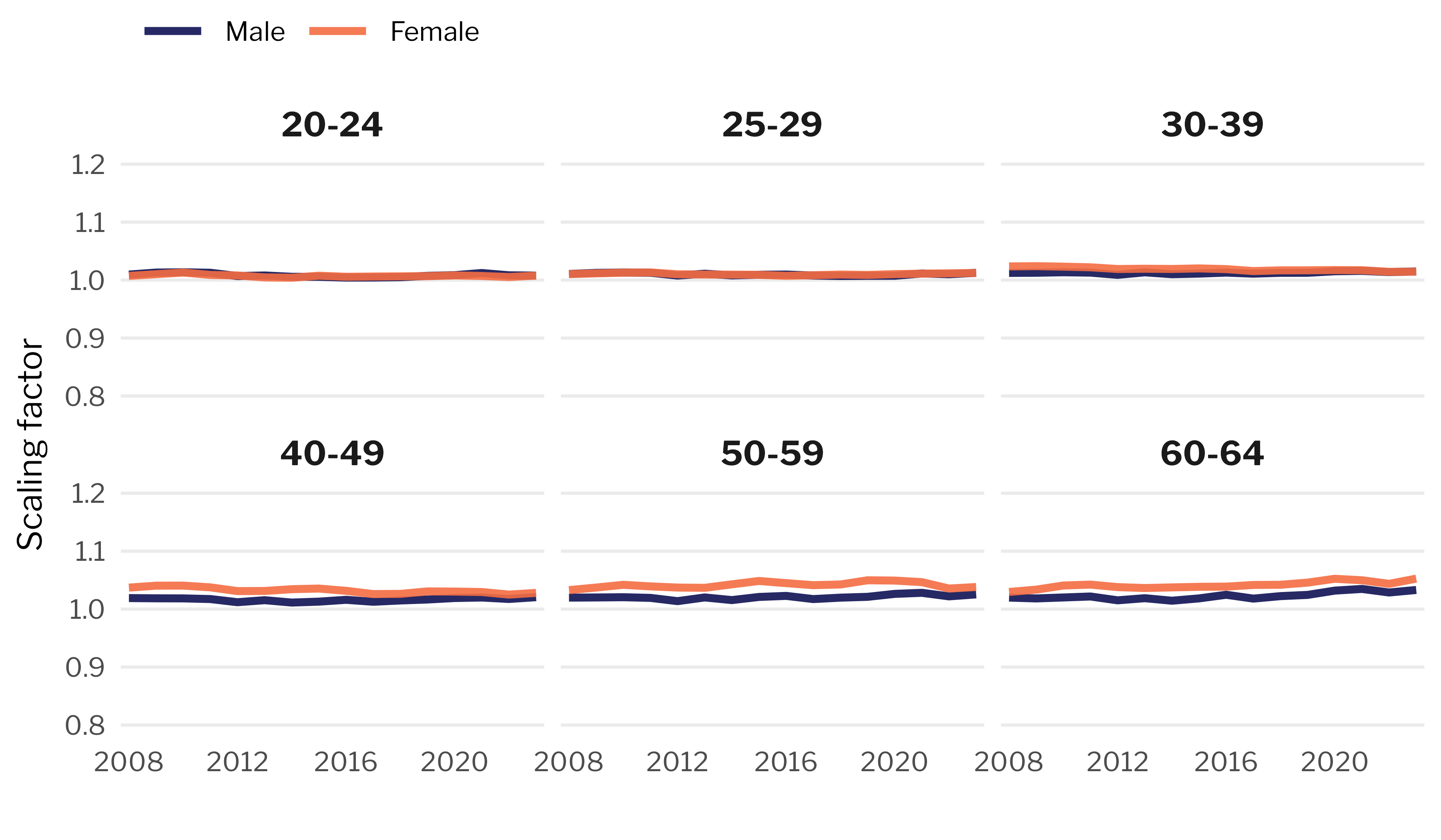
To avoid picking an arbitrary year, I average the obtained scaling factors over the 2008-2023 period for each age group.

Similarly, I rescale pre-2004 wages to account for the exclusion of firms with fewer than 10 employees. These micro-firms tend to pay lower wages than larger establishments, so pre-2004 surveys systematically overstate average wages. The scaling factor follows analogous logic:

$$ M_{t}^{\text{size},(s)} = 1 + s_{\text{micro},t}^{(s)}\big(r^{(s)}-1\big) $$

where (by sex $(s)$):

$r^{(s)} = W_{\text{micro}}^{(s)} / W_{10+}^{(s)}$ = wage ratio for micro-firms (1-9 employees) relative to firms with 10+ employees
$s_{\text{micro},t}^{(s)}$ = sex-specific employment share of micro-firms across covered sectors

Computing these components requires combining multiple data sources. For the employment share $s_{\text{micro}}^{(s)}$, I proceed in two steps. First, I obtain sector-specific employment shares by firm size from the Spanish Ministry of Social Security (Estadística de Empresas Inscritas en la Seguridad Social). This dataset provides annual counts of employment by firm size categories for all NACE Rev. 2 sectors covered in the 2008-23 Structure of Earnings Survey (except public administration), which I use to compute sector-year specific micro-firm shares $s_{\text{micro},k,t}$ for each sector $k$.

Second, I weight these micro-firm shares by sex-specific sectoral employment shares from the Labour Force Survey:

$$ s_{\text{micro},t}^{(s)} = \sum_{k} \omega_{k,t}^{(s)} \cdot s_{\text{micro}, k, t} $$

where $\omega_{k,t}^{(s)}$ is the share of sex $s$'s employment in sector $k$ at year $t$, computed only over the sectors B-S covered by the Structure of Earnings Survey.

For the wage ratio $r^{(s)}$, I rely on published tabulations from the 2006 Structure of Earnings Survey (see Gráfico 38 here), which provides average wages by firm size and sex. The ratio is derived by solving:

$$ W_{\text{all}}^{(s)} = s_{\text{micro}}^{(s)} \cdot W_{\text{micro}}^{(s)} + (1 - s_{\text{micro}}^{(s)}) \cdot W_{10+}^{(s)} $$

for $r^{(s)} = W_{\text{micro}}^{(s)} / W_{10+}^{(s)}$.

Since the firm size adjustment must be applied to the 2002 survey, the key assumption is again that this scaling factor remains stable over time. The resulting scaling factors are shown in Figure 2, which displays the evolution of $M_{t}^{\text{size},(s)}$ over time by sex, and confirms its stability. These adjustments are more substantial than the public administration correction, reflecting the relatively large share of employment in small firms and their lower average wages. For the analysis, I average the obtained scaling factors over the entire 2013-2023 period for each sex.

Figure 2: Scaling factors for micro-firms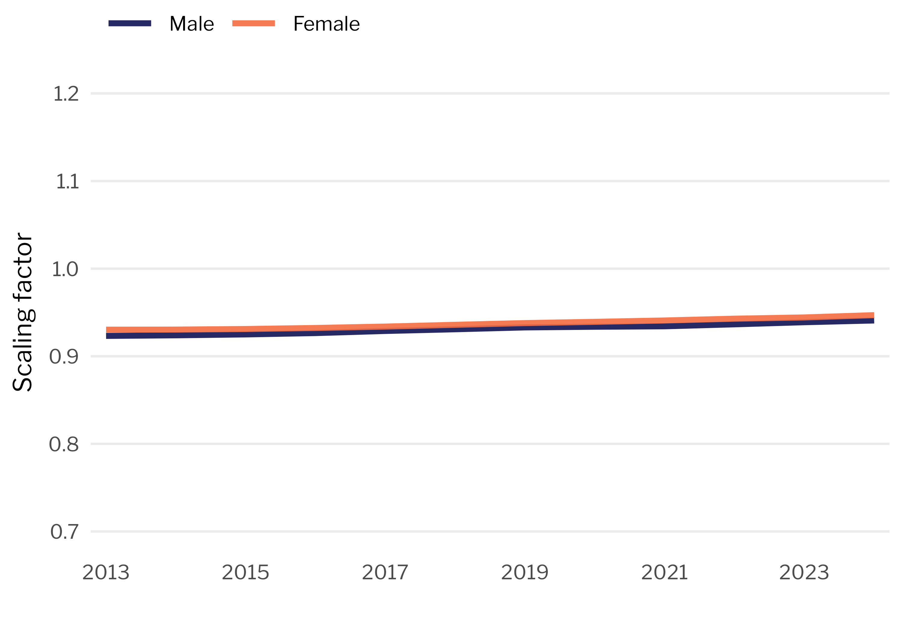 exclusion

With these two adjustments in place, we are ready to proceed with the Lexis expansion as described above.

Cohorts and indexing#

With single-year ages, cohorts are straightforward:

$$c = t - a$$

I group individual cohorts into decades (1950s, 1960s, etc.). For each cohort decade $d$, the average wage at age $a$ is just:

$$\bar{w}(a, d) = \frac{1}{|C_d|} \sum_{c \in C_d} w^{Lexis}(c, a)$$

I index everything relative to the 1960s cohort at age 40 separately by sex. That is, an index of 80 at age 30 means that the cohort earns 80% of what the 1960s cohort of the same sex earned at age 40.

Results and discussion#

The results are shown in Figure 3. For males, the profile suggests that each successive cohort has experienced weaker wage growth throughout their working lives. By age 35, men born in the 1980s earned almost 10% less in real terms than the 1960s cohort did at the same age. The 1990s cohort has failed to catch up and seems to be on a similar trajectory to those born in the 1980s, with earnings about 9% lower than what the 1970s cohort earned at comparable ages.

For females, the picture is different but hardly encouraging. Recent cohorts show signs of convergence, with women born in the 1990s reaching parity with the 1970s cohort by their late-20s and outperforming the 1980s cohort by their early-30s. In this context, however, "convergence" means matching or slightly exceeding wage levels from decades ago. I will let the reader decide whether this warrants celebration.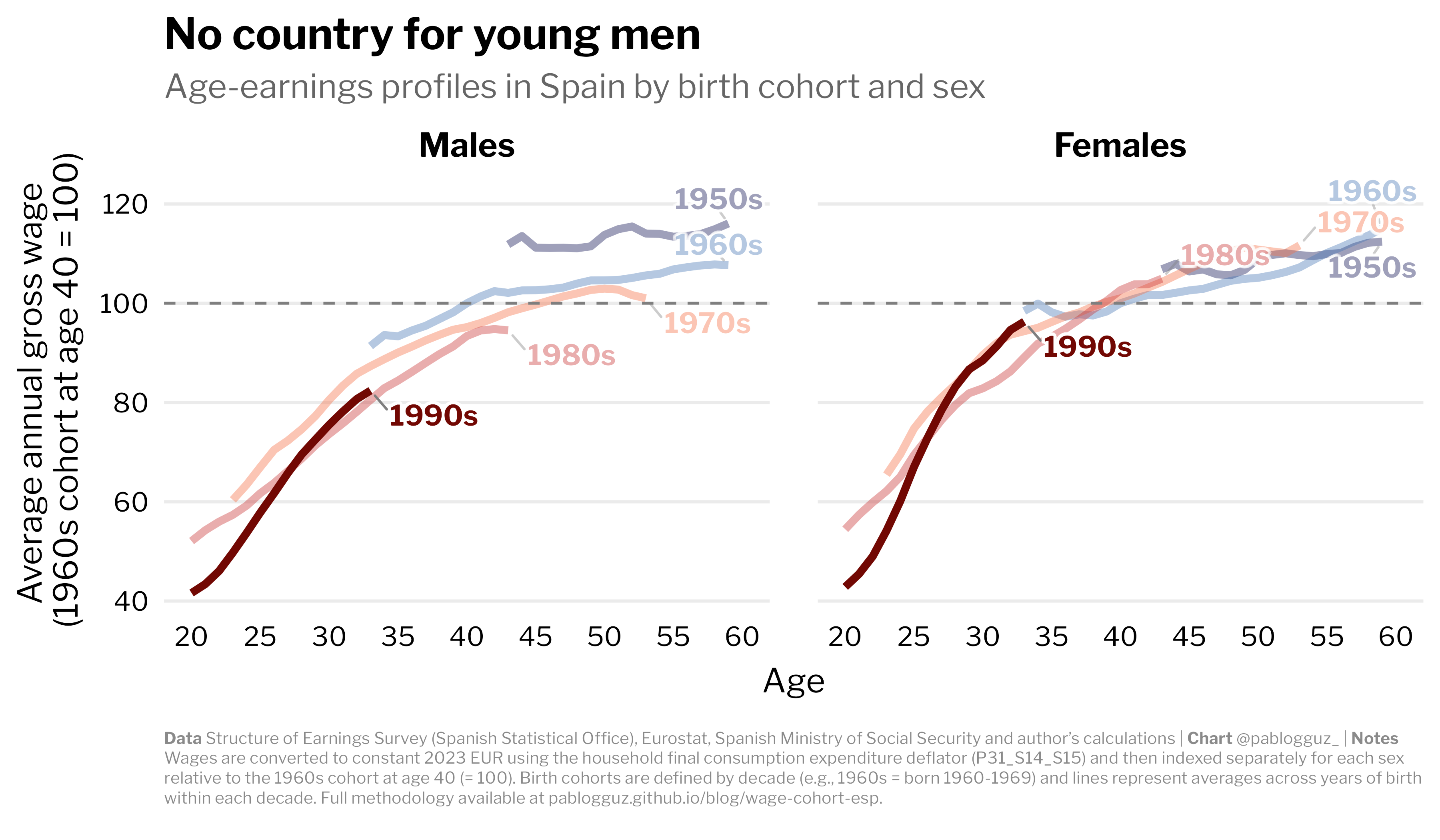

As a result, the gender wage gap has narrowed substantially across cohorts. Figure 4 shows the female-to-male wage ratio by cohort and age. Women born in the 1990s earn 88 cents for every euro their male counterparts make at ages 25 and above, up from 83 cents for the 1970s cohort at similar ages. In other words, the gender wage gap has shrunk by roughly 30% in two decades.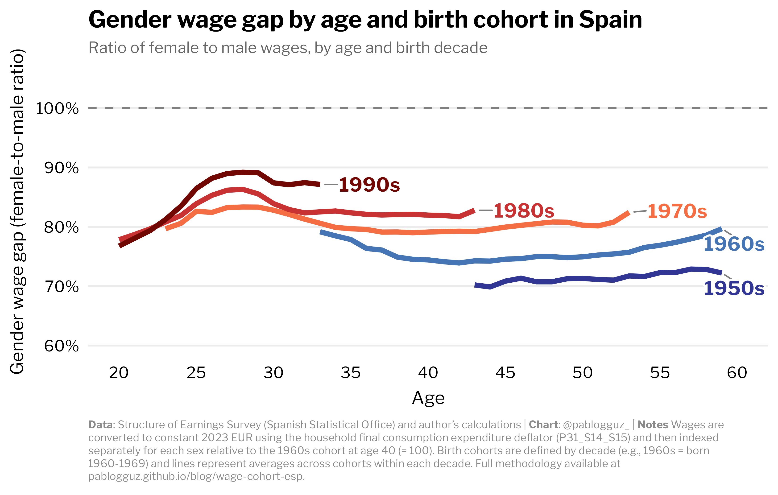

Discussing the root causes of this divergence is beyond the scope of this post, but it would be an interesting avenue for future work. I speculate on a couple of mechanisms below.

First, one could think about structural change. The 2008 financial crisis and subsequent Eurozone crisis disproportionately affected sectors of the economy that were dominated by male workers, particularly in construction and manufacturing (see here and here). These sectors never fully recovered, and if labour supply was absorbed by low-skill jobs in service sectors like retail and hospitality, this could have contributed to the observed wage stagnation for younger cohorts. Descriptively, one indeed sees that manufacturing employment has been in steady decline since the early 1990s, while construction employment collapsed after 2008 and has only partially recovered since then (see Figure 5). Employment in accommodation and food services has increased in relative terms, but there does not seem to be any sex-specific pattern. A Rodrik-style within/between decomposition of wage growth by sex could tell us how much of the cohort gap comes from within-sector wage changes vs. shifts across sectors.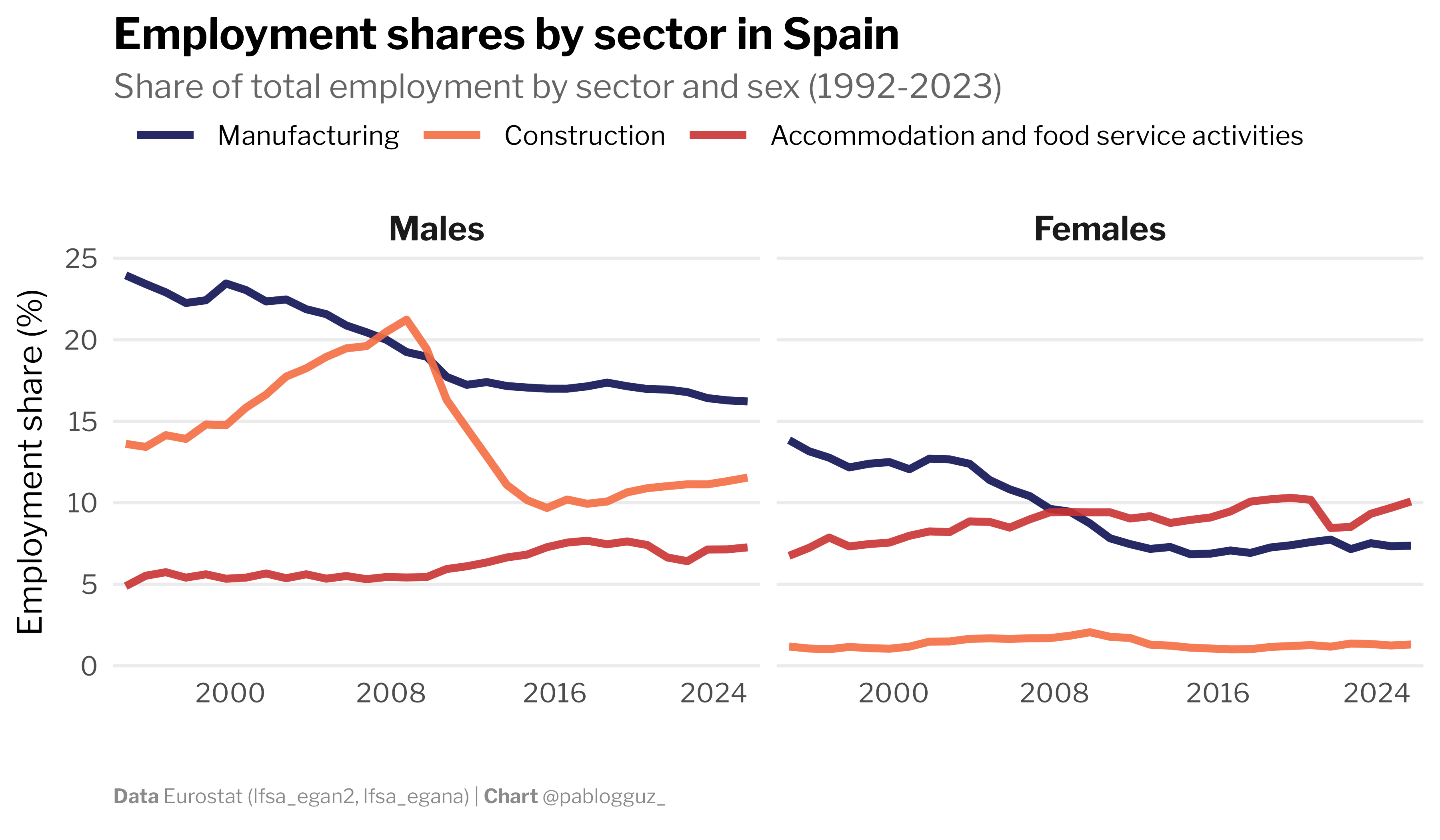

Second, the analysis in this post focuses on average wages, but cohort gaps might reflect differences in hours worked and job intensity. In Spain, output per hour has increased over the last decades, but these improvements have not translated into higher average wages – instead, they have been absorbed by reductions in hours worked (see here). The gender divergence could also reflect a disproportionate reduction in male hours among younger cohorts.

Whatever the mechanisms, these numbers tell a grim story. The absence or even reversal of improvements in labour market outcomes across generations represents the collapse of an implicit contract that held for decades: work hard and society will reward you with opportunities for upward mobility. That promise seems to be evaporating. A dysfunctional labour market, housing costs that previous generations never faced relative to their income, and the fiscal burden of an ageing population have created a perfect storm. Spain's younger generations have inherited an economy that has turned against them.

Contemporary Spain is no country for young men. And increasingly, no country for the young.

I tested the sensitivity of the results by including an adjustment for the partial coverage of public administration when computing the sectoral employment shares, assuming a range of plausible coverage rates of the General Regime. The results are virtually unchanged.