Creating maps with ineAtlas
Pablo Garcia Guzman
2026-04-24
Source:vignettes/mapping-with-ineatlas.Rmd
mapping-with-ineatlas.RmdThis vignette demonstrates how to use ineAtlas to create
choropleth maps of socioeconomic indicators across Spanish
municipalities.
Load required packages
First, let’s load the required packages. We will use the mapSpain
package to get the municipality geometries.
Get municipality data
Let’s fetch income data for all Spanish municipalities for the year 2022:
# Get municipality level income data
mun_data <- get_atlas(
    category = "income",
    level = "municipality"
) %>%
    filter(year == 2022)

# Preview the data
head(mun_data)
#> # A tibble: 6 × 11
#>   mun_code mun_name        prov_code prov_name  year net_income_pc net_income_hh
#>   <chr>    <chr>           <chr>     <chr>     <dbl>         <dbl>         <dbl>
#> 1 01001    Alegría-Dulant… 01        Araba/Ál…  2022         15116         38507
#> 2 01002    Amurrio         01        Araba/Ál…  2022         16011         39221
#> 3 01003    Aramaio         01        Araba/Ál…  2022         20201         51737
#> 4 01004    Artziniega      01        Araba/Ál…  2022         15651         38089
#> 5 01006    Armiñón         01        Araba/Ál…  2022         15755         36433
#> 6 01008    Arratzua-Ubarr… 01        Araba/Ál…  2022         22484         58424
#> # ℹ 4 more variables: net_income_equiv <dbl>, median_income_equiv <dbl>,
#> #   gross_income_pc <dbl>, gross_income_hh <dbl>
Get municipality geometries
Now we’ll get the municipality geometries from
mapSpain:
# Get municipality geometries
mun_map <- esp_get_munic_siane() %>%
    # Join with our income data
    left_join(
        mun_data,
        by = c("LAU_CODE" = "mun_code")
    )

# Preview the joined data
glimpse(mun_map)
#> Rows: 8,132
#> Columns: 18
#> $ codauto             <chr> "01", "01", "01", "01", "01", "01", "01", "01", "0…
#> $ ine.ccaa.name       <chr> "Andalucía", "Andalucía", "Andalucía", "Andalucía"…
#> $ cpro                <chr> "04", "04", "04", "04", "04", "04", "04", "04", "0…
#> $ ine.prov.name       <chr> "Almería", "Almería", "Almería", "Almería", "Almer…
#> $ cmun                <chr> "001", "002", "003", "004", "005", "006", "007", "…
#> $ name                <chr> "Abla", "Abrucena", "Adra", "Albanchez", "Albolodu…
#> $ LAU_CODE            <chr> "04001", "04002", "04003", "04004", "04005", "0400…
#> $ geometry            <MULTIPOLYGON [°]> MULTIPOLYGON (((-2.775594 3..., MULTI…
#> $ mun_name            <chr> "Abla", "Abrucena", "Adra", "Albanchez", "Albolodu…
#> $ prov_code           <chr> "04", "04", "04", "04", "04", "04", "04", "04", "0…
#> $ prov_name           <chr> "Almería", "Almería", "Almería", "Almería", "Almer…
#> $ year                <dbl> 2022, 2022, 2022, 2022, 2022, 2022, 2022, 2022, 20…
#> $ net_income_pc       <dbl> 11635, 10927, 9316, 10464, 11054, 9761, 10103, 120…
#> $ net_income_hh       <dbl> 25522, 22066, 25639, 21030, 23237, 26991, 19494, 2…
#> $ net_income_equiv    <dbl> 16511, 15129, 14206, 14958, 15436, 15267, 13757, 1…
#> $ median_income_equiv <dbl> 15050, 13650, 12950, 13650, 14350, 13650, 12250, 1…
#> $ gross_income_pc     <dbl> 13305, 12361, 10650, 11885, 12457, 11545, 11311, 1…
#> $ gross_income_hh     <dbl> 29187, 24962, 29311, 23885, 26187, 31924, 21823, 3…
Create a choropleth map
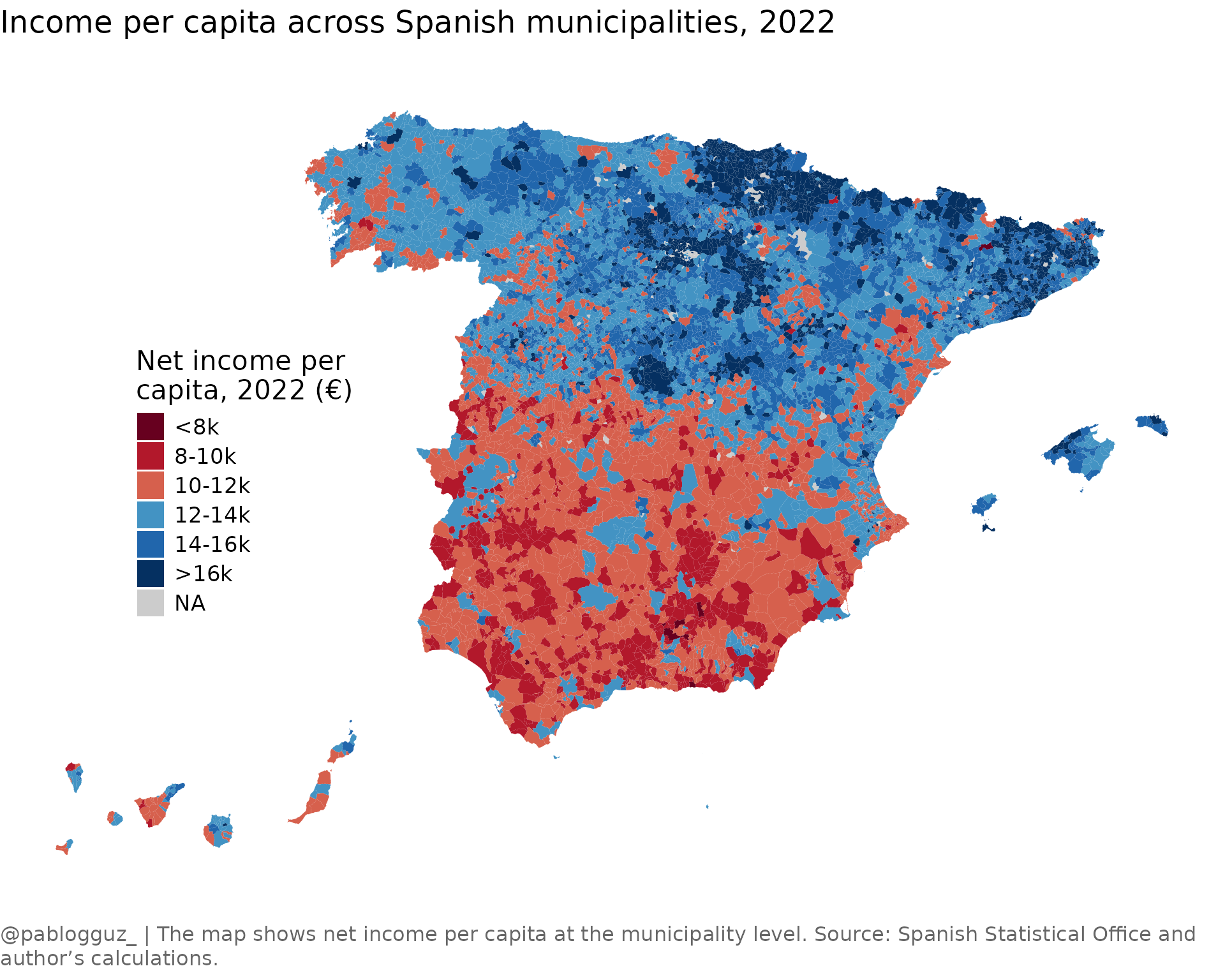
Let’s create a map showing net income per capita across Spanish municipalities:
# Create the map
ggplot(mun_map) +
    geom_sf(
        aes(fill = cut(net_income_pc,
            breaks = c(-Inf, 8000, 10000, 12000, 14000, 16000, Inf),
            labels = c("<8k", "8-10k", "10-12k", "12-14k", "14-16k", ">16k")
        )),
        color = NA
    ) +
    labs(
        title = "Income per capita across Spanish municipalities, 2022",
        caption = "@pablogguz_ | The map shows net income per capita at the municipality level. Source: Spanish Statistical Office and author's calculations."
    ) +
    scale_fill_manual(
        name = "Net income per \ncapita, 2022 (€)",
        values = c("#67001F", "#B2182B", "#D6604D", "#4393C3", "#2166AC", "#053061"),
        na.value = "grey80"
    ) +
    theme_void() +
    theme(
        text = element_text(family = "Open Sans", size = 16),
        plot.title = element_text(size = 18, margin = margin(b = 20)),
        legend.position = c(0.2, 0.5),
        plot.caption = element_textbox_simple(
            size = 12,
            color = "grey40",
            margin = margin(t = 20),
            hjust = 0,
            halign = 0,
            lineheight = 1.2
        )
    )
Identifying high and low income areas
Let’s find the top 10 municipalities by net income per capita:
mun_data %>%
  arrange(desc(net_income_pc)) %>%
  select(mun_name, net_income_pc) %>%
  head(10) %>%
  mutate(
    net_income_pc = round(net_income_pc, 2)
  )
#> # A tibble: 10 × 2
#>    mun_name                 net_income_pc
#>    <chr>                            <dbl>
#>  1 Pozuelo de Alarcón               29258
#>  2 Oroz-Betelu/Orotz-Betelu         25780
#>  3 Goñi                             25532
#>  4 Matadepera                       24814
#>  5 Bolvir                           24812
#>  6 Boadilla del Monte               24748
#>  7 Palau de Santa Eulàlia           24437
#>  8 Madremanya                       24190
#>  9 Vilamòs                          24052
#> 10 Brull, El                        23957
And the bottom 10:
mun_data %>%
  arrange(net_income_pc) %>%
  select(mun_name, net_income_pc) %>%
  head(10) %>%
  mutate(
    net_income_pc = round(net_income_pc, 2)
  )
#> # A tibble: 10 × 2
#>    mun_name            net_income_pc
#>    <chr>                       <dbl>
#>  1 Odèn                         6274
#>  2 Torre del Burgo              6277
#>  3 Manjarrés                    7146
#>  4 Huesa                        7603
#>  5 Darro                        7712
#>  6 Guadahortuna                 7757
#>  7 Iznalloz                     7777
#>  8 Palmar de Troya, El          7779
#>  9 Albuñol                      7949
#> 10 Palomas                      8036